Capital Asset Pricing Model (CAPM): Definition, Formula, and Examples
The Capital Asset Pricing Model (CAPM) i has significantly influenced the way investors evaluate and price assets. Developed in the 1960s by William Sharpe, John Lintner, and Jan Mossin, the CAPM provides a framework for understanding the relationship between risk and expected returns on investments.
Article Contents
Key Takeaways
| Takeaway | Description |
| Definition | CAPM is a financial theory that describes the relationship between risk and expected return of an asset. It suggests that investors should be compensated with higher expected returns for taking on additional risk. |
| Formula | E(Ri) = Rf + βi × (E(Rm) – Rf), where E(Ri) is the expected return, Rf is the risk-free rate, βi is the asset’s beta (systematic risk), and E(Rm) – Rf is the market risk premium. |
| Beta (β) | Beta measures the volatility of an asset’s returns relative to the overall market. It quantifies the asset’s systematic risk that cannot be diversified away. |
| Security Market Line (SML) | The SML is a graphical representation of the CAPM equation, plotting the expected return on the y-axis and the asset’s beta on the x-axis. Assets above the SML are undervalued, and those below are overvalued. |
| Applications | CAPM is used for asset valuation, portfolio optimization, determining the cost of equity capital, and evaluating investment performance. |
| Assumptions | CAPM assumes efficient markets, rational investors, a single-period model, and the ability to hold a well-diversified portfolio. |
| Limitations | CAPM has been criticized for not accounting for size, value, and momentum effects, leading to alternative models like the Fama-French Three-Factor Model. |
What is the Capital Asset Pricing Model?
The Capital Asset Pricing Model (CAPM) is a widely accepted financial theory that describes the relationship between the risk of an asset and its expected return. It is based on the principle that investors should be compensated for taking on additional risk, and it provides a framework for determining the appropriate expected rate of return for an asset, given its level of risk.
At the heart of CAPM is modern portfolio theory – all about risk, return and diversification. In short, this concludes that investors should only expect to be ‘compensated’ for risk they take that cannot be diversified away – systematic risk.
What is the formula for CAPM?
The CAPM formula is expressed as:
E(Ri) = Rf + βi × (E(Rm) – Rf)
Where:
- E(Ri) is the expected return on the asset or investment
- Rf is the risk-free rate of return (typically the return on government bonds)
- βi (beta) is the measure of the asset’s systematic risk relative to the market
- E(Rm) is the expected return on the market portfolio. The market portfolio is a theoretical (but almost investable) portfolio that comprises holdings in all risky assets in proportion to their market values.
In practice, CAPM is applied to the narrower world of public equities and ‘the market’ is an all-market stock index such as the FTSE All Share.
Components of CAPM Calculation
Risk-Free Rate (Rf)
The risk-free rate represents the return that an investor can expect from an investment with no risk, such as government bonds or Treasury bills. It serves as the baseline return for any investment, as investors should expect a higher return for taking on additional risk
.
Beta (βi)
Beta is a measure of an asset’s systematic risk, which is the risk that cannot be eliminated through diversification. It quantifies the volatility of an asset’s returns relative to the overall market. It is measured statistically using observed market returns. The actual computation is:
β = Covariance (i,m) / Variance (m)
Covariance (i,m) being the covariance between the investment returns and the market returns. You can see here that it is a measure of relative risk. It is NOT the same as correlation, but correlation does come into it. If a security has zero correlation with the market, it will have a beta of zero.
It can also be visualized conceptually as the slope of the line of best fit, when plotting excess market returns vs excess security returns:

Note that the axes are the surplus return of the market (Rm) and the Security (Rs) over and above the risk-free rate. The reason being that we are only interested in the excess returns achieved by taking risk.
Also note, that by taking the line of best fit we ignore the ‘scattering’ of the plot points around the line which is the returns uncorrelated to the market. That is, the extent to which a scatter point is not ‘on the line’ is due to stock specific risk that can be diversified away.
A beta greater than 1 indicates that the asset is more volatile than the market, while a beta less than 1 suggests that the asset is less volatile.
Market Risk Premium (E(Rm) – Rf)
The market risk premium is the additional return that investors expect to receive for investing in the market portfolio, which includes all risky assets, over the risk-free rate. It represents the compensation for taking on market risk (systematic risk that cannot be diversified away).
Graphing CAPM
The Capital Asset Pricing Model can be graphically represented using the Security Market Line (SML). The SML is a graphical representation of the CAPM equation, plotting the expected return on the y-axis and the asset’s beta on the x-axis.
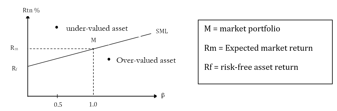
The slope of the SML is determined by the market risk premium (E(Rm) – Rf), and the y-intercept represents the risk-free rate (Rf). Assets that fall above the SML are considered undervalued, as their expected returns are higher than what the CAPM predicts, while assets below the SML are considered overvalued, with expected returns lower than the CAPM prediction.
Interpreting CAPM in Finance
The Capital Asset Pricing Model provides valuable insights for investors and portfolio managers in finance:
- Asset Valuation: The CAPM helps determine the appropriate expected return for an asset based on its level of risk. This information can be used to assess whether an asset is overvalued or undervalued relative to its risk.
- If an asset is fairly valued, then it should sit on the SML; it generates a fair level of return for its level of systematic risk (beta). An asset that is overvalued (expensive) will sit below the line. If markets are efficient, its price should fall, so all other things being equal its % return will rise until it sits squarely and fairly on the SML. And vice versa for undervalued assets.
- Portfolio Optimization: By considering the risk and expected return of individual assets, the CAPM can assist in constructing an optimal portfolio that maximizes returns for a given level of risk or minimizes risk for a desired level of return.
- Cost of Capital: The CAPM is widely used by corporations to estimate their cost of equity capital, which is a crucial component in evaluating potential investments and making capital budgeting decisions.
- Valuation (determining the Ke in a DCF model): Corporate financiers use CAPM in valuation models to determine the Cost of Equity (Ke, being Rf + β(Rm-Rf)).
- Generally, Rm-Rf is taken, in practice, to be in the range of 4-6% – which is a wide range! CAPM can’t give a definitive model – it’s too simplistic, most would argue – but it does give specific parameters which can be modelled and varied in sensitivity analysis to assess its impact on valuation.
- Performance Evaluation: The CAPM serves as a benchmark for evaluating the performance of investment managers and portfolios. By comparing the actual returns to the expected returns predicted by the CAPM, investors can assess whether their investments are generating appropriate returns for the level of risk taken.
Assumptions and Limitations of CAPM
While the Capital Asset Pricing Model provides a useful framework for understanding risk and return, it is important to acknowledge its underlying assumptions and limitations:
- Efficient Markets: The CAPM assumes that markets are efficient, meaning that all relevant information is quickly reflected in asset prices. However, in reality, markets can be inefficient, and prices may not always accurately reflect all available information.
- Investor Rationality: The model assumes that investors are rational and risk-averse, making decisions based solely on expected returns and risk. However, investor behavior can be influenced by various psychological and behavioral factors.
- Single-Period Model: The CAPM is a single-period model, which means it does not account for changes in risk and expected returns over time.
- Single Factor Model: CAPM is a single factor model – relying on Beta. Multi-factor model variations can also be used to disaggregate risk and come up with a more granular valuation model. But CAPM is quick, simple and easy to use as a starting point.
- Measurement Challenges: Accurately measuring the risk-free rate, market risk premium, and beta can be challenging, as these inputs may be subject to estimation errors or fluctuations. If beta is measured as a historic statistic, does it necessarily hold strong for future periods? The past is not always a good guide to the future! So many analysts use more complex models to come up with a range of predictive betas.
- Diversification Assumptions: The CAPM assumes that investors can hold a well-diversified portfolio, which may not always be feasible, particularly for individual investors with limited resources.
Despite these limitations, the Capital Asset Pricing Model remains a widely used and influential theory in finance, providing a useful framework for understanding risk and expected returns.
Empirical Evidence and Criticisms of CAPM
While the Capital Asset Pricing Model has been widely accepted and applied in finance, it has also faced criticism and been subject to empirical testing. Some of the key empirical findings and criticisms include:
- Size Effect: Empirical studies have shown that small-cap stocks tend to outperform large-cap stocks, even after adjusting for risk using the CAPM. This suggests that the model may not fully capture all relevant risk factors.
- Value Effect: Research has found that value stocks (those with low price-to-book ratios) tend to generate higher returns than growth stocks (those with high price-to-book ratios), which is not fully explained by the CAPM.
- Momentum Effect: Studies have demonstrated that stocks with strong past performance tend to continue outperforming in the short term, a phenomenon not accounted for by the CAPM.
- Fama-French Three-Factor Model: Eugene Fama and Kenneth French developed an alternative model that includes two additional risk factors – size (small-cap vs. large-cap) and value (high book-to-market vs. low book-to-market) – to address some of the empirical shortcomings of the CAPM.
Despite these criticisms, the CAPM remains a foundational model in finance, and its insights continue to influence asset pricing and portfolio management practices.
Estimating Inputs for CAPM Calculation
To apply the Capital Asset Pricing Model, investors need to estimate the required inputs: risk-free rate, beta, and market risk premium. Here are some common approaches:
- Risk-Free Rate (Rf): The risk-free rate is typically approximated using the yield on long-term government bonds, such as 10-year Treasury bonds in the United States, or 10-year Gilts in the UK. Remember that these investments are not entirely risk-free, but they are uncorrelated to equity markets, and so the equity beta is zero! (no systematic risk)
- Beta (β): Beta can be estimated using historical data by regressing the returns of an asset against the returns of a broad market index. Alternatively, investors can use published beta estimates from financial data providers.
- Market Risk Premium (E(Rm) – Rf): The market risk premium is often estimated using historical data by calculating the average excess return of the market over the risk-free rate. Investors can also use forward-looking estimates based on market expectations and economic forecasts.
It is important to note that these inputs are estimates and subject to uncertainty and potential errors. Investors should regularly review and update their estimates to ensure the accuracy of their CAPM calculations.
Example Analyses for CAPM
To illustrate the practical application of the Capital Asset Pricing Model, let’s consider the following examples:
Example 1: Evaluating an Investment Opportunity
Suppose an investor is considering investing in Company XYZ’s stock. The risk-free rate is currently 3%, and the expected return on the market portfolio is 10%. Company XYZ’s beta is 1.2.
Using the CAPM formula:
- E(Ri) = Rf + βi × (E(Rm) – Rf)
- E(Ri) = 3% + 1.2 × (10% – 3%)
- E(Ri) = 3% + 8.4%
- E(Ri) = 11.4%
Based on the CAPM calculation, the expected return on Company XYZ’s stock should be 11.4%. If, based on current prices, the total return is only, say, 8% then it is not compensating investors fairly for the risk take. It is overvalued. risk associated with the investment.
Example 2: Calculating the Cost of Equity Capital
A company is evaluating a new project and needs to determine its cost of equity capital to assess the project’s viability. The risk-free rate is 4%, the market risk premium is estimated to be 6%, and the company’s beta has been measured at 1.5.
Using the CAPM formula:
- Cost of Equity Capital = Rf + β × (E(Rm) – Rf)
- Cost of Equity Capital = 4% + 1.5 × (6%)
- Cost of Equity Capital = 4% + 9%
- Cost of Equity Capital = 13%
The company’s cost of equity capital, calculated using the CAPM, is 13%. This information can be used to evaluate the potential profitability of the new project and make informed capital budgeting decisions.
By applying the CAPM formula and considering its components, investors and financial professionals can make more informed decisions about investment opportunities, capital budgeting, and risk management. However, it is important to recognize the model’s assumptions and potential limitations, and to use it in conjunction with other financial analysis tools and market insights.