Portfolio Optimisation in Excel
If you would like a copy of the Excel spreadsheet containing the data and analysis below, feel free to contact Greg: Greg.m@capitalcitytraining.com
It was in the summer that I blogged about my diversified portfolio – noting how my ‘random weighting’ might be as good as anything scientifically optimised, given that I don’t have a crystal ball. But evidence has it that although returns are hard to predict, correlations and covariance relationships do tend to hold in the near future as they have done in the past. What this means in practical terms is that, although we cannot ‘manage’ the returns of our investment portfolios, we can shape our portfolios to look ‘well balanced’ and sensible by looking at historic variances and covariances.
I’m going to show you the steps in finding the minimum variance frontier for a portfolio of investments. From the outputs we can identify my minimum variance portfolio, and the one that gives me the best risk/return ratio – with hindsight!
Step 1: Get your investment funds or stocks data
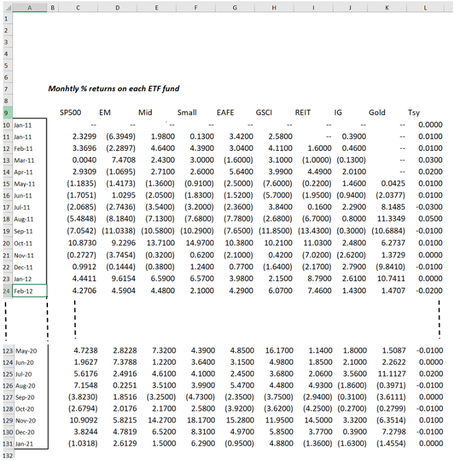
My investable ‘risky’ portfolio comprises 9 ETFs, and then there’s my ‘risk-free’ short term treasuries to help me balance my risk. You can see in Figure 1 what those ETFs cover. I use 10 years of monthly data (Jan 2011 – 2021) for each (excl.the Gold ETF which didn’t start until May 2011). These are returns net of ongoing charges, so they are truly achievable.
Figure 1: the raw data

Step 2: Use the Excel Data Analysis Toolpak to extract the risk data
The key data required for optimisation is the variance / covariance of the returns of each investment.
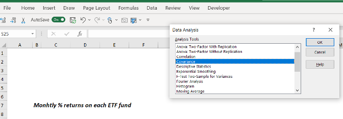
Firstly, if you cannot see “Data Analysis” on the Data menu ribbon, as below, then select: File>>Options>>Add-Ins>> and then ‘Manage Excel Add-ins’ to select the Data Analysis tool kit. This will help you do all the statistical analysis you might ever want!
Figure 2: Selecting the tool to create a Var/Covar matrix in Excel


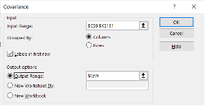
It is then a simple case of selecting the Covariance option: the Input Range being the fund data, and the Output range is the location you choose for the results table.

Figure 3 : the result

I have taken the liberty of adding two columns for the mean returns (monthly and the effective annual rate) and the weights from my ‘random portfolio’ discussed last blog. The grey area is not filled out by the Excel Analysis pack, but it’s just a symmetry of information – you need to complete it for the matrix multiplication to follow.
Step 3: a quick comp
With some simple matrix multiplication you can then determine the portfolio variance. The great thing is that you don’t need the ‘special’ matrix multiplication formulae in Excel – and, in fact, I much prefer the more transparent =SUMPRODUCT() which does the same thing. You can see above in Figure 3 that the calc of the portfolio variance comes in two steps: i) a row of each Weight * (Sum of Covariances * weights) then ii) add up the nine results. Clearly shown in Figure 3.
So, here are our summary stats:

Step 4: Using Solver to find minimum risk for a set of given returns
Here’s the magic bit that Excel can help us with. The Solver add-in is a multi-factor optimisation tool that can use mathematical algorithms to find a solution to a problem with multiple constraints, such as find the weights of a multi-asset portfolio that will give a 5% return with the lower possible variance…… get the idea?
We can ask Solver to find the min-var portfolio for returns of, say, 3%,4%,5%,6%,7%,8% and anything in-between. If the return is achievable, Excel will find a min-var solution.
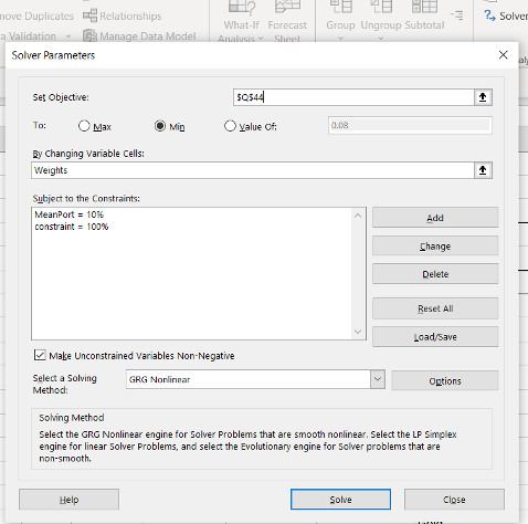
To make it work, I will also define a variable “constraint” that is calculated as the sum of the individual weights, and will specify that these must add up to 100%. Here’s what the Solver parameters look like for setting the target return at 10% (and cell Q44 is the portfolio StdDev).

You run this for “MeanPort” (average return) being 4%, then 5%, then 6% etc, and each time saving the results. This is what I get:

The minimum variance portfolio is the one with the 5.77% standard deviation and a 6% return, and the ‘optimum’ is the one with the best return to risk ratio which is the 8% return portfolio. Try plotting the mean returns and StdDev on a chart….. it will look familiar!
That’s it. A very technical ‘learning’ blog, but a nugget for the investors of you out there.
